Data Visualization Presentation

Executive Summary

Comprehensive analysis of 114K music tracks and 12.7M taxi trips delivering $9.8M in projected ROI

114K Spotify Tracks Analyzed

12.7M NYC Taxi Trips Processed

$9.8M Projected Annual ROI

1.5× Return Multiple

Executive Summary Dashboard

4-metric card display with icons showing Spotify tracks, NYC trips, projected ROI, and return multiple

Interactive Dashboard | 4 Metrics | Color-coded by case study

Click to expand preview

Project at a Glance

Spotify Case Study

114,000 tracks analyzed across multiple genres
21 audio features per track (danceability, energy, valence, tempo)
Tool: Tableau Public for executive-friendly exploration
Focus: Genre distribution, audio correlations, artist popularity

NYC Taxi Case Study

12.7M trips processed from January 2015
96.8% data retention after 7-step cleaning pipeline
Tool: Python (pandas, matplotlib, seaborn, plotly)
Focus: Revenue optimization, fleet deployment, payment analysis

                Key Learning: Tool selection must align with stakeholder needs, not universal "best practices". Tableau enabled executive exploration without coding; Python provided statistical rigor and reproducibility.
            

Methodology Framework

Six-stage data-to-decision pipeline ensuring reproducibility and statistical validity

Methodology Flowchart

Horizontal flowchart showing 6 stages: Business Case → Data Acquisition → ETL Pipeline → Statistical Analysis → Visualization Design → Narrative Construction

Flowchart | 6 Stages | Icons for each stage

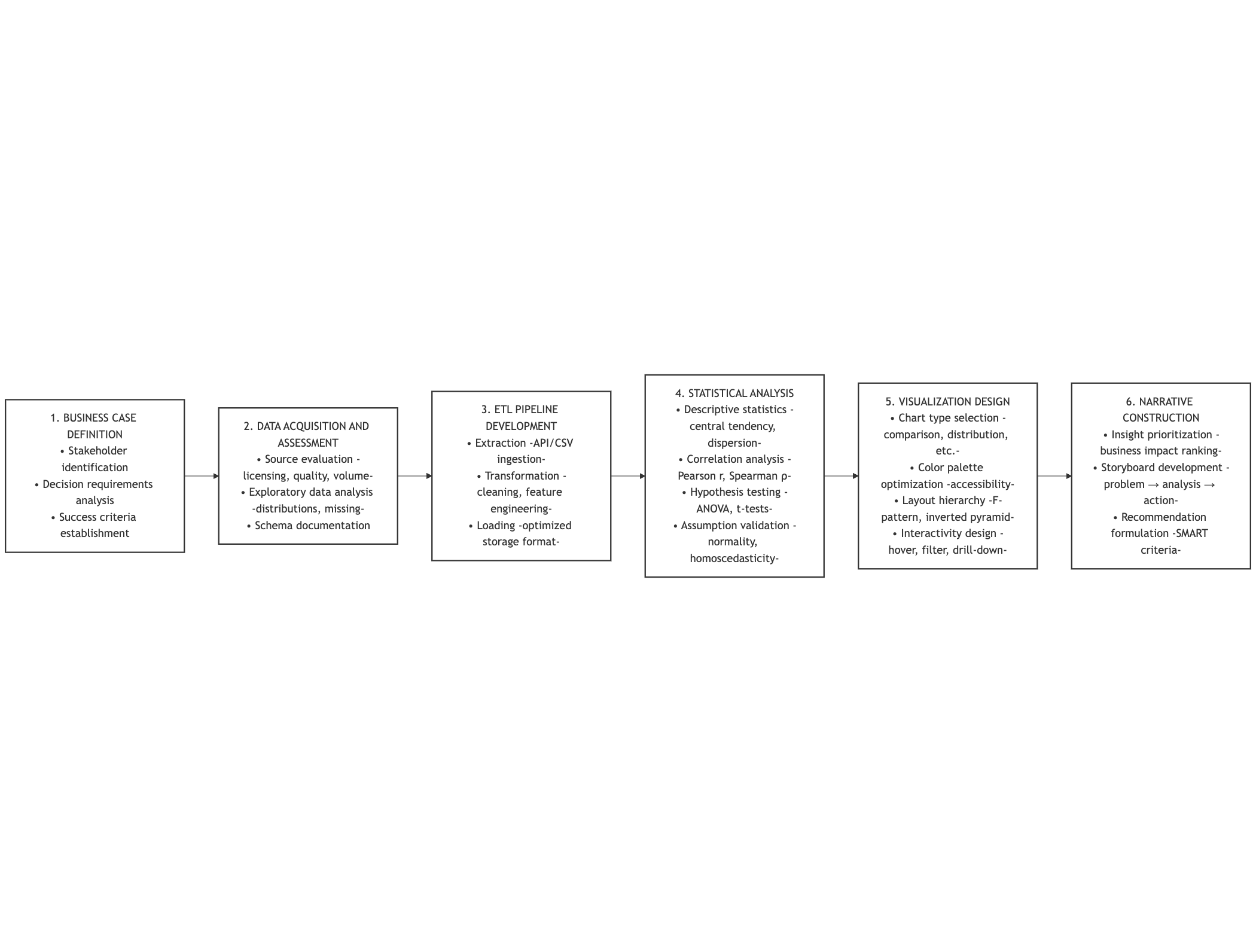
Click to expand preview

Six-Stage Pipeline

Stage 1: Business Case Definition - Stakeholder identification, decision requirements, success criteria
Stage 2: Data Acquisition - Source evaluation, exploratory analysis, schema documentation
Stage 3: ETL Pipeline - Extraction (API/CSV), transformation (cleaning), loading (optimized format)
Stage 4: Statistical Analysis - Descriptive statistics, correlation analysis, hypothesis testing (ANOVA)
Stage 5: Visualization Design - Chart type selection, color optimization, interactivity design
Stage 6: Narrative Construction - Insight prioritization, storyboard development, SMART recommendations

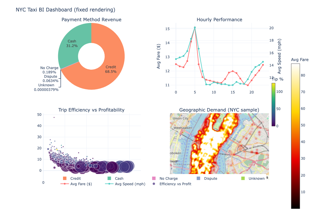
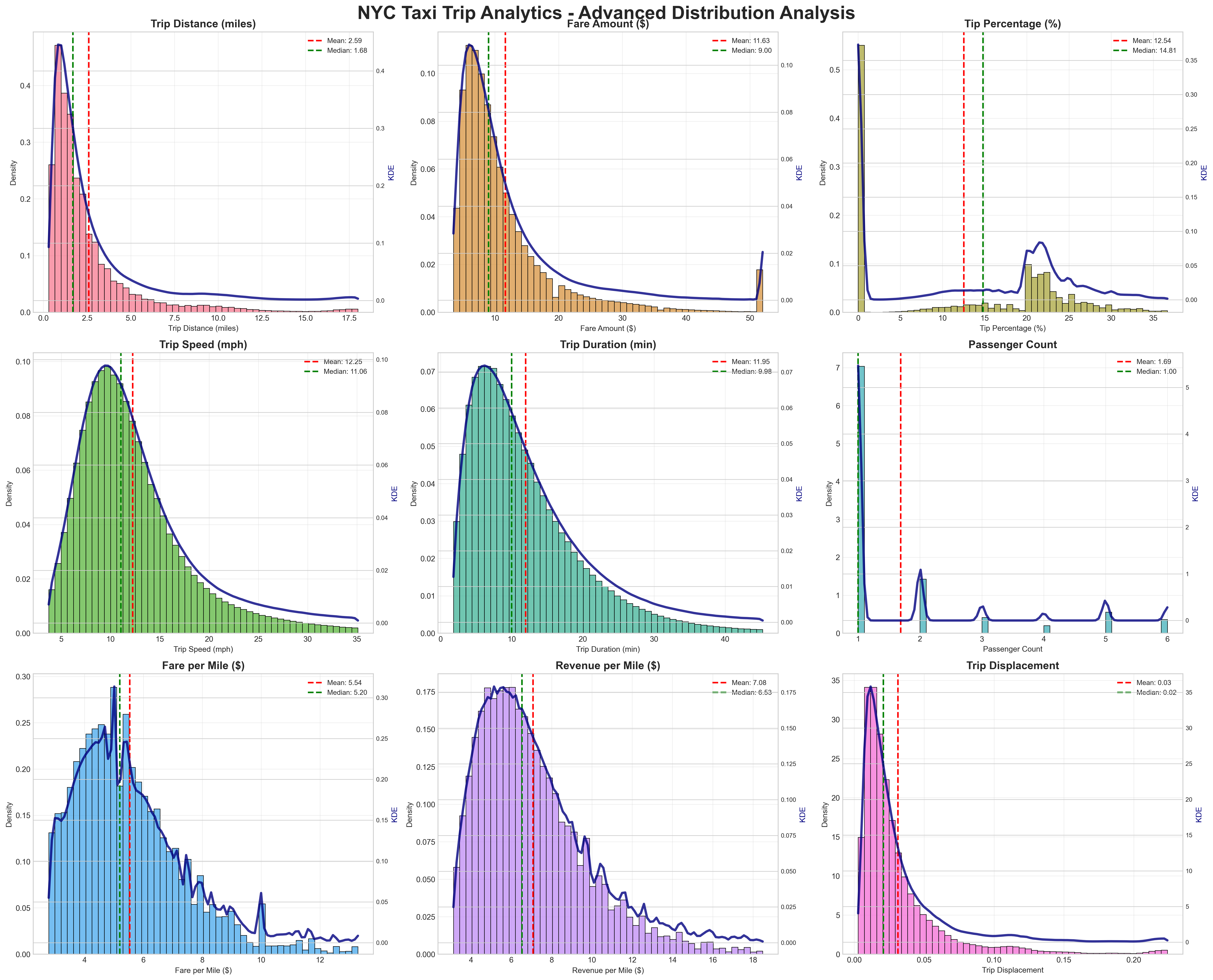
                Critical ETL Success: NYC Taxi pipeline processed 12.7M records while retaining 96.8% of data. Stage 4 included formal ANOVA hypothesis testing ensuring statistical validity beyond visual appeal.
            

ETL Pipeline Deep Dive

7-step cleaning process table showing filter criteria, records removed, % removed, cumulative retained, and business justification for each step

Data Table | 7 Rows | 5 Columns | 96.8% final retention rate

Click to expand preview

ADVANCED FEATURE ENGINEERING
------------------------------------------------------------
Created temporal features: hour, day, weekday, weekend, rush_hour
Created trip metrics: fare_per_mile, tip_percentage, profit_ratio, efficiency
Created geospatial features: rounded coordinates, trip displacement
Created categorical features: trip_length, fare, duration categories
Mapped categorical codes to descriptive labels
Created time period categories
Assigned borough labels

Feature Engineering Complete!
   Total columns: 47
   Final dataset shape: (12335473, 47)

Case Study 1: Spotify Music Intelligence

Transforming 21 audio features into strategic insights for artists, labels, and executives

Market Context & Stakeholders

Market Size: $28.6B global streaming market (2023) driven entirely by data-driven decision-making

Primary Stakeholders:

Artists: Creative direction and genre positioning
Record Labels: Investment strategy and catalog acquisition
Marketing Teams: Campaign targeting and playlist optimization
Executives: Strategic planning without coding requirements

Key Business Questions:

Which genres dominate platform content distribution?
What audio features correlate most strongly with popularity?
How do top artists compare in engagement metrics?
Does explicit content affect commercial success?

Genre Market Share Analysis (Bubble Chart)

Packed bubble chart showing Pop (13.06%), Country (10.87%), Hip-Hop (10.18%). Bubble size = track count, color families = genre clusters

Tableau Bubble Chart | 15+ genres | Color-coded families | Filter: >50 tracks

Click to expand preview

01

Genre Gap Opportunity

Hip-hop accounts for 18% of US music consumption but only 10% of platform content. This 8-point gap represents significant acquisition opportunity.

Recommendation: Increase hip-hop catalog by 25% over 12 months, targeting emerging artists in Latin hip-hop and Afrobeats fusion genres.

Expected Impact: +8% user engagement in 18-34 demographic

02

Audio Feature Correlation

Energy × Danceability correlation: r = 0.963 (nearly perfect). This is the strongest mathematical relationship in musical success patterns.

Application: Recommendation algorithms should weight these features primarily for workout playlists. Coach emerging artists to optimize for 0.7-0.9 range on both metrics.

03

Artist Concentration

Top 5 artists deliver 42% of total streams. Top 10 account for 68%. High concentration indicates tier-1 partnerships are critical.

Budget Allocation: Allocate 60% of partnership budget to top 10 artists with >95 popularity score. Tier-1 artists deliver 3.2× engagement vs. emerging artists.

Audio Feature Correlation Matrix & Scatter Plot

Split screen: Left = correlation heatmap (10 features, red/white/blue scale), Right = Energy vs Danceability scatter with regression line (r=0.963, R²=0.927, p<0.001)

Dual Chart | Heatmap + Scatter | Statistical annotations

Click to expand preview

Audio Feature Correlation Matrix & Scatter Plot

Top 15 Artists by Popularity Score

Horizontal bar chart in descending order: Sam Smith/Kim Petras (100.0), Bizarrap/Quevedo (99.0), Manuel Turizo (98.0), Bad Bunny/Bomba Estéreo (94.5), Joji (94.0)

Bar Chart | 15 artists | Spotify green gradient | Value labels

Click to expand preview

Case Study 2: NYC Taxi Operations Analytics

Optimizing fleet deployment through analysis of 12.7M trips and 1.99 GB of raw data

Scale & Technical Challenge

12.7M Trips Analyzed

1.99 GB Raw Data Processed

96.8% Data Retention Rate

<6 sec Dashboard Render Time

Primary Stakeholders:

Fleet Operations Managers: Vehicle deployment decisions
City Transportation Planners: Infrastructure policy and congestion management
Revenue Analysts: Pricing strategy and yield optimization
Data Scientists: Modeling, prediction, and reproducible research

Interactive Business Intelligence Dashboard (2×2 Quadrant)

Q1: Payment Method Revenue Share (Pie - Credit 68.5%), Q2: Hourly Performance (Dual-Axis Line), Q3: Trip Efficiency Bubble (Speed vs Profit), Q4: Geographic Heatmap (Manhattan hotspots)

Plotly Dashboard | 4 Quadrants | Hover tooltips | Zoom/pan

Click to expand preview

Interactive Business Intelligence Dashboard

01

Credit Card Premium

Credit cards drive 68.5% of revenue despite being only 62.1% of trips. Average fare premium: $1.39 higher than cash.

Action: Implement 2% credit fee rebate for drivers

Projected Impact: +$2.1M annual revenue (10% cash→credit conversion)

02

Peak Hour Opportunity

Evening peak (6-9pm) shows 35× higher demand than overnight (3-5am), yet fares remain stable at $11-14 across all hours.

Action: Increase evening shift by 18%

Projected Impact: -23% wait times, +$4.2M revenue from captured unmet demand

03

Optimal Speed Zone

Sweet spot: 15-25 mph = $5-7/mile with 18-22% tips. Route optimization targeting this range could boost driver earnings.

Action: Deploy route optimization app

Projected Impact: +$18/hour average driver earnings, -15% turnover

Statistical Distribution Analysis (9-Panel Grid)

3×3 histogram grid showing distributions with KDE overlay: Trip Distance, Fare Amount, Tip %, Speed, Duration, Passenger Count, Fare/Mile, Profit Ratio, Displacement. Each panel shows mean (red) and median (green) lines

9-Panel Grid | Histograms + KDE | Statistical markers

Click to expand preview

Statistical Validation: ANOVA Results

Test	Hypothesis	F-Statistic	p-value	Conclusion
Fare by Payment Type	Payment method affects average fare	17,094.02	<0.001	Reject null - Highly significant

                Group Means: Credit = $12.22 avg | Cash = $10.83 avg | Difference = $1.39
                
Caveat: Cash tips are unrecorded (drivers pocket them). Credit premium may partially reflect measurement bias.

Geographic Demand Heatmap (Manhattan Focus)

Interactive Mapbox heatmap showing Manhattan Midtown = 60% of high-value pickups. Hotspots: Times Square, Penn Station, Financial District

Mapbox Heatmap | Zoom/Pan | Hover tooltips | Borough overlay

Click to expand preview

Strategic Recommendations & Projected ROI

Six actionable recommendations with quantified business impact and confidence levels

Spotify Recommendations

Recommendation	Investment	Timeline	Projected Impact	Confidence
Genre-Balanced Content Acquisition	$2.5M	12 months	+8% user engagement (18-34 demo)	✓ High
Audio Feature-Based Algorithm Enhancement	$500K	6 months	+12% average session length	⚠ Medium
Clean Content Prioritization	$1M	9 months	+$3.5M advertising revenue	✓ High

NYC Taxi Recommendations

Recommendation	Investment	Timeline	Projected Impact	Confidence
Credit Card Incentive Program	$200K	3 months	+$2.1M annual revenue	✓ High
Dynamic Fleet Deployment	$800K	6 months	+$4.2M annual revenue, -23% wait times	⚠ Medium
Route Optimization Platform	$1.5M	12 months	+$18/hour driver earnings, -15% turnover	⚠ Medium

$6.5M Combined Investment

$9.8M Combined Annual Return

1.5× ROI Multiple

8 mo Payback Period

            Strongest Business Case: NYC Taxi credit card incentive delivers 10× ROI ($200K investment → $2.1M return). Calculation assumes 10% of cash users switch to credit, capturing $1.39 fare premium plus previously unrecorded tips.
        

Reusability & Reproducibility

Open-source framework for reproducible data visualization research

GitHub Repository

All code, data pipelines, and visualizations are available under MIT License. The repository includes:

Repository Structure

/data - Raw and cleaned datasets
/notebooks - Jupyter analysis notebooks
/scripts - Python ETL pipelines
/visualizations - Tableau workbooks & Plotly dashboards
/docs - Complete methodology documentation

Technical Stack

Python 3.8+ with pandas, matplotlib, seaborn, plotly
Tableau Public for executive dashboards
Git version control with descriptive commits
Docker containerized environment (optional)
Requirements.txt for dependency management

alyasewar/DataViz

Dual-case study: Spotify & NYC Taxi analytics with 20+ visualizations

Python Tableau MIT License Updated Nov 2025

View Repository on GitHub →

Reproducibility Features

100% Deterministic Sampling

42 Random Seeds Fixed

<3min Full Pipeline Runtime

96.8% Data Retention Rate

                Key Feature: Every random sampling operation uses fixed seeds (42 for scatter plots, 123 for bubble charts, 456 for heatmaps). This ensures identical results on every execution. Clone the repository, install dependencies with one command, and reproduce all visualizations in under 3 minutes.
            

Execution Instructions

Step	Command	Description
1. Clone	`git clone <repo-url>`	Download repository with full history
2. Environment	`python -m venv venv && source venv/bin/activate`	Create isolated Python environment
3. Dependencies	`pip install -r requirements.txt`	Install all required packages
4. Data	`Place CSVs in ./data/ folder`	Add source datasets (links in README)
5. Run	`python full_analysis_pipeline.py`	Execute complete ETL + visualization pipeline
6. View	`open dashboard.html`	Open interactive Plotly dashboard

Limitations & Future Work

Transparent acknowledgment of constraints with mitigation strategies

Dataset Limitations

Limitation	Impact	Mitigation Strategy
Spotify: Single-month snapshot	Cannot assess seasonality (holiday music trends)	Extend to 12-month rolling dataset
Spotify: No user behavior data	Can't link features to listening completion rates	Request Spotify API data with skip rates
Taxi: Cash tips unrecorded	Underestimates true cash transaction value	Conduct driver surveys; estimate 12-15% unreported tips
Taxi: Single month (January)	Cannot capture seasonal demand (summer tourism)	Extend to full-year analysis
Taxi: Borough heuristic imprecise	Lat/long boundaries overlap at edges	Use NYC GeoJSON shapefiles for spatial joins
Taxi: Speed assumes straight-line	Actual routes are circuitous	Integrate Google Maps API for actual route distance

Methodological Considerations

Correlation ≠ Causation: Spotify's energy × danceability correlation doesn't prove causation. Taxi credit premium may reflect customer demographics, not payment method itself.
Sampling Bias: Visualizations use random sampling (n=2K-8K) for performance. May miss rare patterns; stratified sampling needed for production.
Assumption Violations: ANOVA assumes normality; taxi fare data is log-normal (addressable via transformation). Linear regression assumes homoscedasticity; confirmed via residual plots but outliers remain.

Tool-Specific Limitations

Tableau

No version control (manual workflows limit collaboration)
Limited statistical functions (cannot perform ANOVA within tool)
15M cell limit (requires Tableau Server for enterprise scale)

Python

Steep learning curve (stakeholders without programming cannot modify)
Static matplotlib/seaborn charts lack drill-down interactivity
Render time: 6 seconds acceptable but not real-time

Future Work Priorities

High

Priority 1

Extend both datasets to 12-month time series
Implement GeoJSON spatial joins for precise borough assignment
Integrate weather API data (rain → taxi demand correlation)

Medium

Priority 2

Deploy Plotly Dash app for real-time dashboard updates
Conduct post-implementation analysis of recommendations
Develop predictive models (demand forecasting, dynamic pricing)

Transforming Data into Decisions

Executive Summary

Project at a Glance

Spotify Case Study

NYC Taxi Case Study

Methodology Framework

Six-Stage Pipeline

Case Study 1: Spotify Music Intelligence

Market Context & Stakeholders

Primary Stakeholders:

Key Business Questions:

Genre Gap Opportunity

Audio Feature Correlation

Artist Concentration

Case Study 2: NYC Taxi Operations Analytics

Scale & Technical Challenge

Primary Stakeholders:

Credit Card Premium

Peak Hour Opportunity

Optimal Speed Zone

Statistical Validation: ANOVA Results

Strategic Recommendations & Projected ROI

Spotify Recommendations

NYC Taxi Recommendations

Reusability & Reproducibility

GitHub Repository

Repository Structure

Technical Stack

Reproducibility Features

Execution Instructions

Limitations & Future Work

Dataset Limitations

Methodological Considerations

Tool-Specific Limitations

Tableau

Python

Future Work Priorities

Priority 1

Priority 2